Reverse-engineering FIFA's secret World Cup algorithm
INT. FIFA HEADQUARTERS - ZURICH, SWITZERLAND - NIGHT An INTERN enters, clutching a printout.INTERNGIANNI INFANTINO’s chair turns slowly, revealing him first in side profile and then head-on.
“Sir, we have the score from Algeria vs. Austria. Somehow, it’s a tie: 3-3.”
GIANNI INFANTINO
“The time has come. Execute option sixty-seven.”
I’m not quite sure that’s how it actually played out, but at some point on June 27
Perhaps early in the morning of June 28 Zurich time.
, 2026, somebody at FIFA finalized the standings of the twelve third-place teams at the 2026 World Cup. The top eight third-place teams, which came from groups B, D, E, F, I, J, K, and L, would continue into the knockout stage. But who would their opponents be?
To answer that, we had to turn to Annexe C of the 2026 FIFA World Cup regulations. In that eighteen-pageFor comparison, FIFA’s regulations regarding the World Cup stadiums take up just one page.
appendix, FIFA laid out which third-place team would fill each of the eight slots in the 32-team knockout bracket depending on which set of eight groups produced qualifying third-place teams. (FIFA calls these sets options; we’ll use the term scenarios.) Since there were twelve groups, but only eight slots, FIFA had to specify slot assignments in different scenarios, explaining the absurd length of Annexe C.
Once we knew which eight groups produced a qualifying third-place team (i.e., which scenario we were in), we could lookThe scenarios (“Options”) in Annexe C are in reverse lexicographic order on the sorted string of qualifying groups—e.g., BDEFIJKL in the scenario that actually happened (Option 67).
through Annexe C to figure out which matchups we were going to get. Despite the ten thousand articles and videos apparently required to explain it to sports fans, this procedure is pretty straightforward: it’s just a lookup table. But nobody seemed to be able to figure out how the lookup table was generated.
“Two-thirds of the 12 first-place finishers are scheduled to face a grab bag of third-place teams based on what’s literally an indecipherable algorithm.” (Nate Silver)To be fair, Silver’s use of “indecipherable” may refer not just to the lookup table but also to the placement of the third-place slots in the 32-team knockout bracket. We don’t tackle the latter problem here at all. That said, @me, Nate.
“It’s unclear exactly how the permutations were decided.” (Sportico)
“I’m guessing from the distinct lack of success at that exact task from the online tools, there is no such algorithm. […] if there was a set of rules that would produce that table and only that table, they wouldn’t need the table.” (Sports StackExchange)
“No-one seems to have been able to reverse-engineer the table to work out exactly why the combinations are determined this way. There is no simple explanatory rule.” (Reddit, r/Aleague subreddit)Today, we’ll do just that.
The laws of the game
Let’s get started by making sure we understand what Annexe C actually tells us. For each group winner (1E, 1A, 1I, 1D, 1G, 1L, 1B, 1K)FIFA uses the notation E1 for the team from Pot 1 in group E, and the notation 1E for the first-place team in Group E. These are often, but not always, the same.
that was to face a third-place team, FIFA prescribed five possible groups that the third-place team might come from: the shaded cells in the table below.
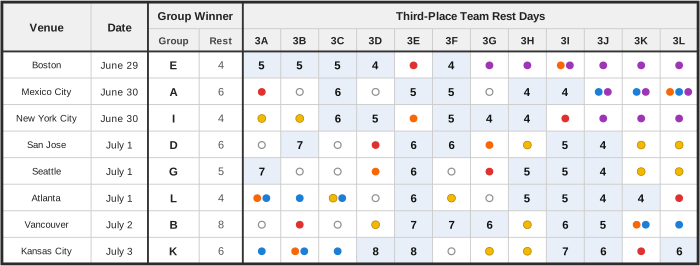
- No round-of-32 rematches of group stage games (red ● circles).
- No potential round-of-16 rematches (orange ● circles).
- No games where one team has fewer than four days of rest (purple ● circles).
- Games where the rest disparity would be three days or more (blue ● circles). The only exception to this rule is the potential 1B-3J matchup.
- Potential quarterfinals rematches (yellow ● circles). These clearly aren’t completely forbidden, but around half of the otherwise-inexplicably-excluded matchups could give rise to potential quarterfinals rematches.
Matching up
For every scenario, FIFA had to choose pairings between the first-place teams and third-place teams. Some scenarios offer few choices: for example, scenarioOption 431 in Annexe C, which prescribes the blue matching.
ABCDGJKL offers only three.
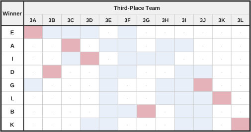
Option 155 in Annexe C.
BCDEFHIJ offers 214 different choices of pairings, the maximum of any scenario.
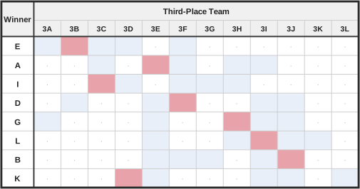
In general, counting perfect matchings is -hard by a famous result of Valiant. The input graphs here are small enough that this doesn’t matter.
there are in each scenario. Multiplying these counts together tells us that there are
possible ways to choose one perfect matching per scenario. So how did FIFA do it?
How FIFA didn’t do it
Before we explain how FIFA did choose the 495 perfect matchings, let’s rule out some plausible-but-wrong explanations. (If you want to skip to the actual explanation, click here.) This will help us better understand the shape of the problem before we present the actual procedure FIFA used.It’s not random
Anybody who’s spent time staring at Annexe CThere are dozens of us. Dozens!
knows instinctively that it isn’t random. But how can we actually argue that it isn’t?
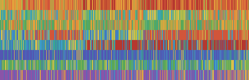
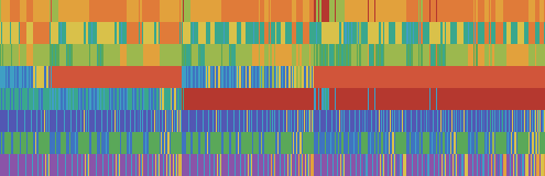
Let’s assign each third-place team (3A-3L) a color. Then we’ll pick a random matching per scenario, and plot the eight qualifying third-place team colors in a column ordered by the first-place team each was matched with.Using the EAIDGLBK row order from the tables above.
Finally, we’ll join together all 495 such columns. When we do that, we get plots that look like this:
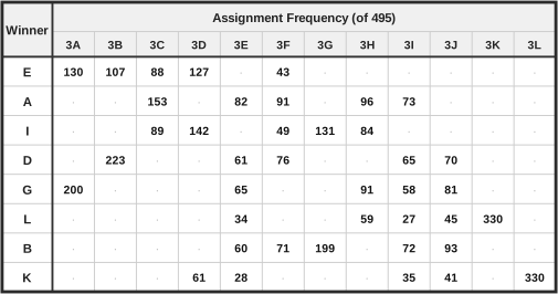
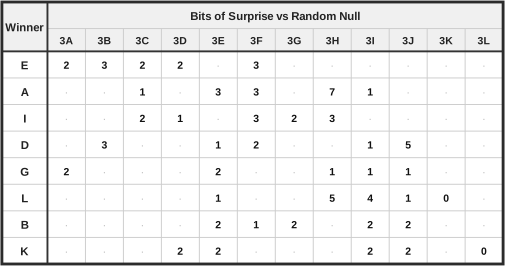
Not forty, since we have two tail probabilities per cell.
tail probabilities.
Now let’s look at Annexe C. Here’s the assignment-frequency table:
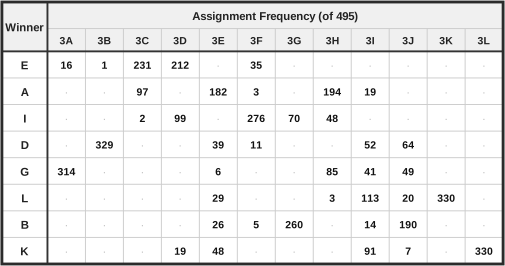
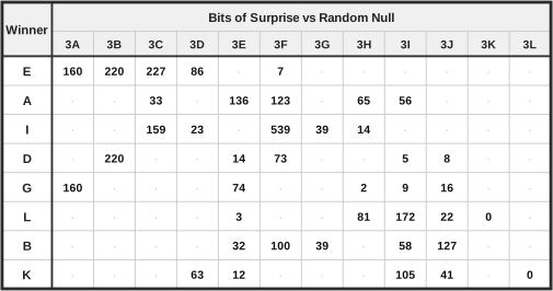
To be fair, we are cherry-picking the most extreme of eighty tail probabilities, so proper accounting deducts bits for selection. I think we can afford it.
is barely even an actual number. No event has ever happened in the history of the observable universe.
Annexe C isn’t random.
It’s not lexicographic
The lone concrete conjecture I found in the wild is from an answer on Sports StackExchange: namely, that the table can be generated by“a simple exercise of filling up a table by picking the first available possibility for each match, going from left to right.”It’s worth being explicit about how the post’s proposed procedure works. We start by picking a scenario. We then make all forced pairings—e.g., if 3L qualifies it has to play 1K—in the given scenario.
Since all scenarios have at least three possible matchings, this step never produces a complete pairing.
Next, we work through the remaining slots by match numberIn other words, first 1E (match M74), then 1I (M77), 1A (M79), 1L (M80), 1D (M81), 1G (M82), 1B (M85), and finally 1K (M87). This does not match the chronological slot order we use in our tables.
from §12.6 of the regulations. For each slot, we simply pick the first available third-place team alphabetically.This is what the post means by “left to right”.
This procedure may not always produce a complete pairing, as it’s possible that earlier choices could leave us with no choices at some later step. If we backtrack appropriately, however, we’ll just end up choosing the lexicographically minimal valid matching. So let’s call that our procedure. Does it match FIFA’s?
The StackExchange post’s author checked this procedure against Options 1 and 2We switch to option numbers temporarily here to help the reader reference Annexe C.
in Annexe C, found it produced the correct matchings, and noted that checking the other 493 would require a script. I wrote a script.Claude Code wrote a script.
It did not go well for the conjecture.Claude Code said it did not go well for the conjecture. I checked Claude Code’s work.
To give the poster some credit, the first seven options in Annexe C agree with the output of this procedure, even though they only checked the first two. The chances of getting Options 3-7 correct if you picked matchings at random are one in 3.9 million, so the poster’s proposed procedure is really, really good! It’s also wrong.
The procedure first fails on Option 8, where the lexicographic rule matches 1L-3H, 1D-3I, and 1G-3J. FIFA, on the other hand, matched 1L-3I, 1D-3J, and 1G-3H, which no “grab the first thing available” rule could produce.
Of course, it’s possible that FIFA processed the slots in some other order. Happily, this is checkable: for each of the slot orderings, we can ask whether FIFA’s matching is the lexicographically-minimal valid matching with respect to that processing order in all 495 options.We also checked lex-max, as well as column-major lex-min and lex-max, across all row and column orderings. It’s important to be paranoid.
No lexicographic rule made it past the first ten options of Annexe C.
It’s not greedy
A slightly-more-sophisticated version of the lexicographic conjecture above is to let the preference order vary per slot. As an example, perhaps for slot 1A’s opponent we prefer 3C to 3F (in order to equalize rest days), but for slot 1I’s opponent we prefer 3F to 3C (which would also minimize rest-day discrepancy). Then the procedure would proceed over slots in some order, with each slot taking its most-preferred still-available qualified third-place team (with look-ahead so nobody gets stranded). The search space here is enormous: match-processing orders times preference profiles is about 1.7 sextillion such procedures, which is way too many to enumerate. It turns out that we don’t have to enumerate, though: we can show that no such procedure can work by looking at revealed preferences. Here’s the idea. Let’s fix a processing order for slots: say EAIDGLBK, as in our tables. In every one of the 495 scenarios, slot 1E gets its first choice of the qualified third-place teams. Now slot 1E can be paired with 3A, 3B, 3C, 3D, or 3F. Looking at Option 4 of Annexe C tells us that slot 1E prefers 3D to 3F, because 3F was available but slot 1E was paired with 3D. Similarly, Option 18 tells us that slot 1E prefers 3C to 3D. Unfortunately, Option 19 tells us that slot 1E prefers 3D to 3C. Hence there can be no consistent global preference for slot 1E if it is processed first. We’ve just ruled out one-eighth of the possible slot-processing orders with a few lines of logic. With a fair few lines of code, we can build up preference graphsNote that if we’re considering the second slot to be processed, we can’t conclude anything about preferences involving the first third-place team to be picked, because it wasn’t available.
for each slot and check to see if any have cycles (which would mean no consistent global preference order).
In fact, every slot’s preferences have cycles which could easily have been found by hand:
- Slot 1A can’t be processed first: it prefers 3F to 3I in Option 327, but prefers 3I to 3F in Option 56.
- Slot 1B swaps 3E/3F preferences between Options 33 and 487.
- Slot 1D swaps 3E/3F preferences between Options 31 and 270.
- Slot 1E swaps 3C/3D preferences between Options 18 and 19.
- Slot 1G swaps 3A/3I preferences between Options 166 and 286.
- Slot 1I swaps 3C/3G preferences between Options 82 and 397.
- Slot 1K swaps 3E/3J preferences between Options 42 and 362.
- Slot 1L swaps 3H/3J preferences between Options 126 and 246.
Implicit in this claim is the fact that every possible matchup is part of at least one valid matching; without that fact, this claim wouldn’t quite be true.
We can run the same trick to verify that FIFA didn’t go column-by-column either.Column-by-column requires a bit more work because columns 3K and 3L can go first/second, since there’s no way to have inconsistent global preferences when you have exactly one choice.
This is perhaps our most important negative result, so let’s make sure we understand exactly what it says. FIFA’s choice of opponent for a slot cannot be a function of just that slot’s options. The same slot, facing the same available third-place teams, picks differently depending on what the other slots face. No procedure that fills in the bracket one match at a time can generate Annexe C. Local optimization is ruled out.
It’s not rest days
We know FIFA cares a great deal about rest days, so it’s worth ruling out a couple of simple algorithms that use that information. Local optimization is out, but perhaps some sort of global optimization survives? First, let’s note that it makes no sense to maximize total rest. This is because total rest is determined entirely by which scenario we’re in: the number of rest days for the group winner is known, and the number of rest days for the third-place team is simply the date of the match minus the date of that group’s finale. Add these up and we get the sum of the dates of the knockout matches minus the sum of the dates of the qualifying groups’ finales, which clearly depends only on which groups qualified. So every single possible matching maximizes (and minimizes!) total rest. But there are other ways to account for rest. Here are two reasonable possibilities:- We could try to pick a matching that maximizes the minimal number of rest days. For example, suppose one of the three matchings in scenario ABCDGJKL gives every third-place team at least five days’ rest, and the other two give one third-place team four days’ rest. Then we’d pick the one with minimum rest five days.
- We could penalize games with four days’ rest a lot, penalize games with five days’ rest a little less, and so on up to eight days’ rest, then try to minimize the sum of these rest penalties.Importantly, we could perhaps penalize games with eight days’ rest more, not less: aren’t commentators always complaining about rust too?
- Only 394 of the 495 prescribed matchings maximize the minimal number of rest days. Even this large number is mostly due to team 3K being forced to play 1L whenever they qualify, which forces the minimal number of rest days to be 4 no matter what valid matching we choose. If we instead considered trying to lexicographically maximize the sorted list of rest days, which tends to equalize rest across the qualified third-place teams, FIFA’s chosen matching gives the best possible list of rest days in only 35 of 495 scenarios.
- There’s no set of meaningful rest penalties such that FIFA’s chosen matching minimizes the sum of the rest penalties in every scenario. For every scenario, the chosen matching gives some inequality of the form where ranges over the other valid matchings in the scenario and , count how many games the matchings , have with rest days. When we write down all these inequalities, we get a linear program whose only solutions are . The -term is meaningless—it’s just a constant extra penalty—and the term is meaningless because is just the total rest, which (as we saw above) is constant once we’ve fixed a scenario. So these degenerate solutions don’t separate any matchings: they tell us nothing at all.
How FIFA did it
The greedy-algorithm refutation above showed that however FIFA picked matchings, it wasn’t purely a local optimization procedure. The rest-days refutation showed that it wasn’t a global optimization procedure based solely on rest days. So let’s enlarge our space of hypotheses. Not all of the forty FIFA-allowed pairings in our table are created equal. Not only are there rest-day discrepancies, there’s also travel distance to consider. Most groups’ third-place matchesThe only glaring exception is Group H, whose final two matches were in Houston and Guadalajara.
took place in cities that were close to one another, allowing us to assign a consistent “third-place team travel penalty” to each potential pairing of third-place team and venue. We might also assign some sort of “rematch penalty” to pairings that could produce quarterfinals or semifinals rematches.
This is starting to look like a per-pairing penalty—or, with the opposite sign, a per-pairing score. So perhaps FIFA’s matchings are just the ones with the best possible sum of scores. Let’s ask the question:
Is there some set of numbers we can put in the forty potential pairings so that every matching prescribed by Annexe C maximizes the total score of its pairings (among all valid matchings for that scenario)?This question, finally, has a positive answer. Here’s one such set of numbers:
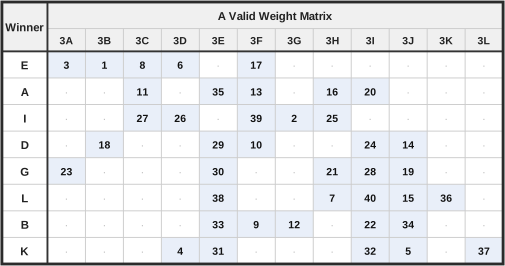
OK, here’s what we did, now that I’ve warned you about getting sidetracked: we picked random initial weights, snapped the weights to the nearest permutation of 1-40, projected back to the feasible cone described by the linear constraints we discuss below, snapped the weights to permutations again, projected again, and so on, hoping that this converges. Sometimes it does!
though, let’s see how these numbers get used in scenario ABCDGJKL, the three-matching example from earlier.
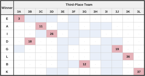
Someone still loves you, Lee Corso.
This is not a coincidence
We should be a little bit suspicious of this solution: forty arbitrary weights is a lot of freedom. Perhaps no matter what choices of matchings FIFA made, it would always be possible to find a set of forty weights that explain the matchings via maximum-weight perfect matching? This turns out to be very, very, very false. Almost no choices of matchings admit weights that do this, and there’s some really neat math that explains why. Here’s how to think about it. Let’s consider an arbitrary weight vector where we number the potential pairings 1-40 from top-to-bottom then left-to-right in the table above. As a concrete example, our valid weight vector from the table above has , , , and . Let’s also form matching vectors, which have ones in the positions corresponding to the eight pairings in the matching and zeroes elsewhere. As a concrete example, the red matching vector has ones at positions 1, 6, 12, 16, 25, 30, 33, and 40, and zeroes everywhere else. Then the sum of weights for a particular matching is simply the dot product of its matching vector with the weight vector. So the fact that the blue matching has maximal sum is equivalent to the two inequalities which we’ll rearrange to read So scenario ABCDGJKL, which has three valid matchings, gives us two half-space constraints (i.e., inequalities of the form ) on the weight vector. Similarly, scenario BCDEFHIJ, which has 214 valid matchings, gives us 213 half-space constraints coming from differences between the maximal matching and the other 213 non-maximal matchings. Across all 495 scenarios, there are a total of 13,939 possible valid matchings, so we get 13,444 half-space constraints in of the form Any other choice of matchings also gives us 13,444 half-space constraints. Unfortunately, the new constraints will not use the exact same set of 13,444 hyperplanes. To see this, let’s suppose that FIFA had instead chosen the green matching in scenario ABCDGJKL. In that case, we’d get the half-space constraints We still get information about the hyperplane normal to , but we don’t get information about the hyperplane normal to : instead, we get information about the hyperplane normal to .The key idea
Let’s step back for a second and figure out where we’re going. We’re trying to argue that a random choice of matchings admitting a valid weight vector is a very unlikely event. To do so, we’re going to want to count, or at least upper-bound, the number of choices of matchings that do admit a weight vector. Now, given a choice of matchings admitting a weight vector, we get a bunch of half-space constraints on said weight vector, so it has to live in the nonemptyThe region is nonempty because we know a vector that lives in it: the weight vector itself!
region in cut out by those half-space constraints.
A different choice of matchings coming from a weight vector gives us different half-space constraints along a different set of hyperplanes. Importantly, the two regions cut out by the constraints are disjoint. This is because the two choices of matchings must disagree in some scenario. If the first choice of matchings has as the maximum-weight matching in that scenario, and the second choice of matchings has , the two matchings disagree about the sign of the dot product coming from the matching-difference vector. Hence the corresponding regions must be disjoint.
This means that we’ve transformed the problem of counting choices of matchings into the problem of counting regions of high-dimensional space cut out by hyperplanes. Believe it or not, this transformation is actually really helpful, because mathematicians have put a lot of work into the latter problem! Now, despite all that work, I don’t know how to calculate the exact number of regions cut out by these particular (joint!) choices of signs and 13,444 hyperplanes. But we don’t need the exact number; we just need a useful upper bound.
Our one saving grace in writing down a useful upper bound is that there aren’t that many hyperplanes in total: letting be the number of valid matchings in scenario , the total number of hyperplanes involved in any constraint for any choice of matchings coming from a weight vector is because every hyperplane involved in a constraint is of the form for matchings , for the same scenario.Note also that gives the same hyperplane—we just need to swap signs—so we don’t need to count negations as well.
These arguments let us write down the very-loose-but-still-very-useful upper bound
The equality here is our disjointness argument above; the inequality comes from forgetting the unnecessary signs.
A two-dimensional illustration
This is a pretty abstract argument, so let’s try to make it a little bit more concrete. Instead of there being 495 scenarios, let’s pretend that there’s just one: scenario ABCDGJKL above, with three matchings (red/green/blue). Let’s also pretend that the red/green/blue matching vectors live in , not , as depicted below: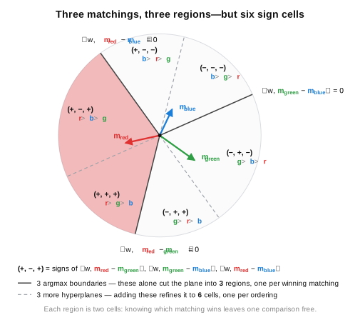
Even though there are eight possible choices for the signs in the inequalities involving the three hyperplanes, two of those eight choices of signs are inconsistent.
So the two-dimensional analogue of our region-counting inequality above reads
In this example, there are fewer different shaded regions (just three) than regions chopped up by hyperplanes (six). In high dimensions, we lose more than just a factor of two; thankfully, we’ve got factors of two to spare.
Numerics
The final quantity in our high-dimensional region-counting inequality above—the nonempty-region count coming from all 390,596 hyperplanes—is easy to upper-bound via the theory of hyperplane arrangements: namely, an inequality due to Schläfli.L. Schläfli, Theorie der vielfachen Kontinuität, ed. J. H. Graf, Zürcher & Furrer, Zürich, 1901, p. 41.
For a centralThat is, an arrangement where all the hyperplanes pass through the origin.
hyperplane arrangement, Schläfli’s inequality gives
In our caseIt’s a good sanity check to compute the Schläfli bound for the , toy case illustrated above and verify that you get six.
, we get the numerical bound
Now, that’s a lot of possible choices of matchings that might come from weight vectors. But earlier, we saw that there are about possible choices of matchings in total. So the chance that a random choice of matchings comes from a weight vector (via taking the maximum-weight matchings) is something like . In other words, there’s a billion billion billion billion billion billion billion billion billion billion billion billion billion billion billion billion billion billion billion billion billion billion billion billion billion billion billion billion billion billion billion billion billion billion billion billion billion billion billion billion billion billion billion billion billion billion billion billion billion billion billion billion to one odds against this happening by random.We can actually improve this bound to around —see the appendix—which would add another ten or eleven “billions” to this figure. But what’s a factor of between friends?
I don’t think a sportsbook would entertain such a wager. This is, to my eyes, the smoking gun: the choice of matchings bears a ridiculously unmistakable mathematical signature. So we can finally claim to have solved the mystery of Annexe C:
FIFA assigned some weights to each of the forty possible pairings, and then recorded for each scenario the perfect matching with the maximum possible sum of weights in Annexe C.
Where’d they come from?
The one remaining question is where these forty free parameters came from. Were they in turn generated from some smaller set?Later on, we’ll see that there are actually only 21 free parameters up to meaningless gauge symmetries. For reference, there are 19 free parameters in the Standard Model. So think of this as an experimental physicist’s answer to how FIFA did it.
What nefarious deeds—it’s FIFA, after all—are concealed within those still-somewhat-mysterious numbers?
I’m not sure that there’s going to be a satisfying answer to this question. For one, we can’t determine exactly what the weights are. The example we gave above is one weight vector that produces the matchings of Annexe C, but there are lots of others.As an example, the 1L-3K and 1K-3L weights can be anything, because they’re the only nonzero entries in their columns.
So we can’t even try to isolate how much FIFA weighted various factors like rest days, travel distance, or potential rematches.
The only satisfying answer would be FIFA themselves saying how they weighted the matches, and that doesn’t seem very likely to happen, does it?
Was the fix in?
Forty parameters of unknown origin also invite the question of whether they could be chosen to favor certain teams. This isn’t all that far-fetched: it was known well before Annexe C was published that Mexico, Canada, and the United States were going to be assigned to groups A, B, and D, respectively. As hosts, they had weaker groups, so were widely expected to end up as teams 1A, 1BRIP to the dream of Canada in Vancouver for the knockouts.
, and 1D. So were these teams favored in, say, expected rest differential?
We tested this hypothesis: namely, we compared each slot’s expected opponent rest under FIFA’s table against the uniform-random baseline. There is no consistent host signal: 1B does get slightly more-tired opponents than chance (by about ten hours, on average), as does 1A (by four hours), but 1D gets fresher ones (about eight hours). So, while FIFA could perhaps have chosen to give the hosts a very slight advantage here, they don’t seem to have done so.
Why weren’t they public?
Setting aside FIFA’s general tendency to be unaccountable, opaque, and corrupt, are there any good arguments against making the weights public? I actually think there are decent arguments for not making the weights public if you’re FIFA. First and foremost, you’re just inviting further criticism of whatever weights you assigned: maybe you decided that flying from Guadalajara to Vancouver wasn’t that bad, or some other sin. Second, you’re inviting people to screw up math,I do this all the time, and I do math for a living.
rather than just screw up a table lookup. Finally, maybe you screwed up the math or the algorithms. I’ve certainly written incorrect implementations of the Hungarian algorithm, so who’s to say FIFA wouldn’t?It wouldn’t be the worst thing they’ve ever done to Hungary.
That said, it would be neat to have them. So if that FIFA intern who actually generated Annexe C is out there, let me know.
Comments? Questions? Corrections? Just want to let me know you enjoyed this? You’re the FIFA intern I mentioned? Interested in having me do nonsense with numbers for you? Email me at [email protected], or check out the code behind this post here.
Appendix: better bounds
There are a few fun ways to improve the quantities in the Schläfli bound that actually give us pretty substantial wins.Improving
The first trick is to reduce the dimension of the weight vectors, since there’s actually a fair bit of degeneracy. There are two forms of degeneracy, plus an overlap between them that we have to make sure not to double-count. First, we can increase all the weights in a given column (i.e., a fixed third-place team) by a constant amount and not change which matchings the weight vector produces. The only matchings we affect are matchings where that team qualified, and all of those see their sum of weights increased by a constant, hence this won’t affect the maximum-weight matching in any scenario. So we can quotient our weight vectors and half-space constraints by the 12-dimensional span of the column vectors. Second, we can do the same thing in a given row. Increasing all the weights in a single row by a constant increases every matching’s total score by that constant, so it again has no effect on the matchings we choose. This lets us quotient by the 8-dimensional span of the row vectors. Unfortunately, these two subspaces intersect in a one-dimensional space spanned by the sum of all weights. So we don’t get a 20-dimensional cutdown, only a 19-dimensional one. But dropping to dimension still helps us enormously, as our Schläfli numerics now becomeImproving
There are two tricks to improve , the number of hyperplanes: deduplication, and single-cycle reduction. Neither buys us too much, but they’re still neat. Recall that our earlier figure came from summing across all scenarios to count the number of vectors of the form where matchings , come from the same scenario. It turns out that not all of these vectors are distinct (up to sign): when we deduplicate, we find that we only have 89,203 distinct matching-difference vectors. That takes us down to We started at Schläfli numerics of , so we’ve already found an extra basically just lying on the floor. We’ve still got one final trick up our sleeves.This trick was found by Claude Fable 5, which is one scary model.
Let’s consider a matching-difference vector . Now, since , are matchings under the same scenario, there’s some permutation of the slots that takes to . This permutation, like all permutations, can be decomposed into disjoint cycles. It turns out that the hyperplane constraint coming from is always redundant if has more than one cycle. This is because we know we don’t care about the constraint unless either or is the maximal matching. If is the maximal matching, then we know that for any single cycle (where the action of permutations on matching vectors abuses notation slightly). But if is the composition of disjoint cycles , then precisely because the cycles are disjoint.
So it suffices to only consider matching-difference vectors coming from matchings that differ by a single cycle. This takes us down to , which gives the best Schläfli numerics I’ve got: the number of choices of matchings that can arise from weight vectors is at most which makes the odds of a coincidence at most . My intuition is that this is still a massive overcount, but I don’t know how to push these techniques any further.