Contents ↑

• Fixing notation
  • The grid
  • Checking our work
  • Divertimento: a Möbius trick
• Combinatorial enumeration
  • The setup
  • The conditions
  • Binary relations
  • Two elements
  • Property checking

Counting and generating inequivalent binary relations

There’s a standard genre of group theory exercise that goes like, “Given a group $G$ acting on a set $X$, count the number of $G$-orbits in $X$.” The intended approach is to use Burnside’s lemma $$|G| \cdot |X/G| = \sum_{g \in G} |\mathrm{Fix}(G)|.$$

For some recent work, I wanted to generate all binary relations on a finite set up to equivalence under permuting the elements of the finite set. In order to check my code, I wanted to count the number of binary relations up to equivalence. This smells like a Burnside’s-lemma problem! Today we’ll solve that problem, then spend some time talking about how to actually generate all binary relations.

Fixing notation

Let $S$ be a finite set, and consider the set $X$ of all binary relations on $S$. Let the permutation group $\mathrm{Aut}(S)$ act on $X$ by relabeling the elements of $S$; if we view a relation $R$ as an $|S| \times |S|$ 0/1-matrix $M_R$ (with ones corresponding to pairs $a, b$ with $aRb$), this action simultaneously permutes the rows and columns of $M_R$. Then $|X/\mathrm{Aut}(S)|$ counts the number of binary relations on a finite set up to relabeling the elements of the set.

In our problem, it’s clear how big $|\mathrm{Aut}(S)|$ is, so all of the work is going to come in figuring out the sizes of the fixed-point sets. A general fact that’s useful in Burnside-lemma problems is that the size of the fixed-point set is constant on conjugacy classes of $G$, so we can collect the summands into conjugacy classes $$\sum_{g \in G} |\mathrm{Fix}(g)| = \sum_{\pi \in \mathrm{Cl}(G)} |\pi| |\mathrm{Fix}(\pi)|.$$

Since $\mathrm{Aut}(S)$ is a finite symmetric group, its conjugacy classes are indexed by cycle type $\alpha = (\alpha_1, \alpha_2, \cdots, \alpha_{|S|})$ as the cycle type ranges over all solutions in nonnegative integers to $\sum_{i = 1}^{|S|} i\alpha_i = |S|$; i.e., over all integer partitions of $|S|$. Calculating the number of permutations of a given cycle type is classical, so the only new ingredient will be calculating the size of the fixed-point set.

The grid

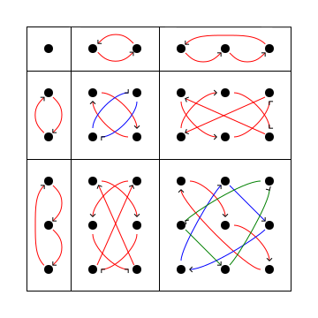
Here it’s helpful to draw a picture. Let’s consider the permutation on six elements $(1)(23)(456)$ with cycle type $(1,1,1,0,0,0)$. This permutation moves the elements of the matrix $M_R$ of a relation as shown below:

How many 0/1-matrices does this permutation fix? Well, the matrix elements along any orbit of this action should be constant, so the permutation fixes $2^{\text{\#} orbits}$ matrices. Okay, so how many orbits are there? Each orbit is contained in a grid cell in the picture above, so we can work cell-by-cell. The number of orbits in a cell of height $h$ and width $w$ is simply $\gcd(h, w)$, so that the total number of orbits of the action of a permutation with cycle type $\alpha$ is simply $\sum_{i,j = 1}^n \gcd(i,j)\alpha_i\alpha_j$.

Checking our work

Putting everything together and doing a tiny bit of cancellation, we get the formula $$\left|X/\mathrm{Aut}(S)\right| = \sum_{\alpha \bot |S|} \frac{2^{\sum_{i,j=1}^{|S|} \gcd(i,j)\alpha_i\alpha_j}}{\prod_{i=1}^{|S|}i^{\alpha_i}\alpha_i!}.$$ For $|S| = 1, 2, \dots$, we get the sequence of counts $$2, 10, 104, 3044, 291968, 96928992, 112282908928, 458297100061728, \dots.$$ This is OEIS sequence A000595, so we’ve done everything correctly.

One fun aspect of the formula above is that it’s a bunch of different powers of two divided by various integers that are definitely not powers of two, yet somehow the total is guaranteed to still be an integer. This is typical of Burnside problems. In fact, in our specific instance we could abandon the binary-relation interpretation, allow our matrices to be 0/1/2-valued, and replace $2$ by $3$ in the formula above, and we’d know we’d still get an integer out. The same goes for 4 or 5, so replacing $2$ by $x$ we get for each $|S|$ a polynomial with rational coefficients that is nonetheless always integer-valued. Here are the first few polynomials for $|S| = 1, 2, \dots$:

$$x, \frac{x^4}{2}+\frac{x^2}{2}, \frac{x^9}{6}+\frac{x^5}{2}+\frac{x^3}{3}, \frac{x^{16}}{24} + \frac{x^{10}}{4}+\frac{x^8}{8}+\frac{x^6}{3}+\frac{x^4}{4}, \dots.$$

We can see that the maximal-degree term comes from the cycle type $(|S|,0,\dots,0)$ and the minimal-degree term comes from the cycle type $(0,\dots,0,1)$. This suggests that the number of inequivalent binary relations should grow as the intuitive guess $2^{n^2}/n!$. A little bit more work is needed to make this precise since it could a priori be the case that there are a large number of slightly-lower-degree terms with smaller denominators that eventually overwhelm the leading-term asymptotics.

Divertimento: a Möbius trick

For large $n$, there’s a cute little way to speed up the summation $\sum_{i,j=1}^n \gcd(i,j) \alpha_i \alpha_j$, which naively takes $O(n^2\log n)$ time (assuming we have $O(1)$ access to the $\alpha_i$). The trick is to find coefficients $c_d$ such that $$\sum_{i,j=1}^n \gcd(i,j) \alpha_i \alpha_j = \sum_{d=1}^n c_d \sum_{i,j=1}^{\lfloor n/d \rfloor} \alpha_{di}\alpha_{dj} = \sum_{d=1}^n c_d \left(\sum_{i=1}^n \alpha_{di}\right)^2.$$ We can compute all the stride-$d$ sums $\sum_{i=1}^{\lfloor n/d \rfloor} \alpha_{di}$ in $O(n \log n)$ time, so the only question left is what the coefficients $c_d$ should be. The easiest way to determine this is to match the coefficients on an arbitrary $\alpha_i\alpha_j$ term. Letting $g = \gcd(i,j)$, we find that we need $\sum_{d | g} c_d = g$. Then we can just apply Möbius inversion to get $$c_d = \sum_{k \mid d} \mu(k)\frac{d}{k} = \phi(d),$$ where $\phi(d)$ is the Euler phi function. Of course, now we need all the $\phi(d)$ values for $1 \le d \le n$, but these can be computed via a sieve-based approach in time $O(n \log \log n)$. Hence the dominant term is the $O(n \log n)$ computation of the stride-$d$ sums, so we’ve shaved off a full factor of $n$ from the computation!

Of course, in our broader context $n$ is so small (since the number of partitions grows quickly enough to overwhelm my computer around $n = 40$) as to make this improvement barely noticeable.

Combinatorial enumeration

What if we want to actually generate representatives of each equivalence class of binary relations on a set of size $n$? It’s one thing to count them; it’s another to actually generate them. The obvious and very stupid strategy is:

1. Enumerate all $2^{n^2}$ binary relations.
2. For each relation, check whether it is equivalent to any relation we’ve already seen.
3. If not, add it to our list.

Thankfully, there is a far more practical approach, due to Read, that avoids equivalence testing almost entirely. Somehow the frustratingly-vague term “combinatorial enumeration” seems to have attached itself to this approach (Read uses the far-better phrase “orderly algorithm”), which is applicable to a number of problems similar to our enumerating-binary-relations focus for today.

The setup

Let us suppose that we have some set $S$ with an isomorphism relation $\cong$, and we want to generate a single representative from each isomorphism class. The setup for an orderly algorithm requires several choices of auxiliary data:

• a partition $S = S_0 \amalg S_1 \amalg \cdots$ of $S$ depending on some integer parameter $q \ge 0$;
• an ordering $\prec$ on $S$;
• a subset $\mathcal{C} \subset S$ of canonical elements of $S$, such that each isomorphism class of $(S, \cong)$ has a unique representative in $\mathcal{C}$; and
• an augmenting operation $A: S_q \longrightarrow S_{q+1}^*$ mapping elements of $S_q$ to $\prec$-ordered lists of elements of $S_{q+1}$.

We should also have some algorithm to determine whether an element of $S$ is canonical, as well as some way of constructing the ordered list $\mathcal{L}_0 = (\mathcal{C} \cap S_0, \prec)$. The data will need to satisfy two conditions–canonical covering and weak monotonicity–which we discuss below. First, though, let us describe how an orderly algorithm proceeds.

The central idea is that we construct the ordered list $\mathcal{L}_{q+1} = (C \cap S_{q+1}, \prec)$ from the ordered list $\mathcal{L}_q$ and the augmentation operation $A$; we can then recover $\mathcal{C} = \mathcal{L}_0 \amalg \mathcal{L}_1 \cdots$. To build $\mathcal{L}_{q+1}$, we begin with the empty list. For each element $e \in \mathcal{L}_q$, we form the list $A(e)$. Then, for each $f \in A(e)$, we append $f$ to $\mathcal{L}_q$ iff $f$ is greater than the $\prec$-maximal element of $\mathcal{L}_q$ and $f \in \mathcal{C}$. The key point is that while we should store $\mathcal{L}_{q+1}$ somewhere as we are building it up, we never need to search over $\mathcal{L}_{q+1}$; we simply have to store the current maximal element instead.

The conditions

Let’s now turn to what conditions we should require of our data for this orderly algorithm to work. First, if all elements of $\mathcal{C} \cap S_{q+1}$ are going to appear in $\mathcal{L}_{q+1}$, then each of them must be generated in some augmentation step. This is what we call canonical covering: namely, that we have $$\mathcal{C} \cap S_{q+1} \subseteq \bigcup_{e \in \mathcal{C} \cap S_q} A(e).$$

This is not enough to ensure that all canonical elements of $S_{q+1}$ actually appear in $\mathcal{L}_{q+1}$, however. We must also choose to append them, which means they must be maximal in the $\prec$-order at the first time they are generated in an augmentation step. Tracing this backwards gives us weak monotonicity: namely, if $e, f \in \mathcal{C} \cap S_{q+1}$ with $e < f$, then we must have

$$\min \left\{x \in \mathcal{C} \cap S_q : e \in A(x) \right\} \preceq \min \left\{x \in \mathcal{C} \cap S_q : f \in A(x) \right\}.$$

It turns out that these two conditions are enough to ensure that the orderly algorithm generates all elements of $\mathcal{C}$. The only argument that needs to be made is that if an element of $S_{q+1}$ is not appended to $\mathcal{L}_{q+1}$ the first time it is generated, then it cannot be appended any subsequent time, which is an easy monovariance argument.

Binary relations

Let us now turn to the specific example of binary relations, following the construction of Read. For a binary relation $R$ on $\{1, 2, \cdots, n\}$, define $$\operatorname{code}(R) = \sum_{1 \le i, j \le n}\mathbf{1}_{[iRj]} 2^{n(n-i)+(n-j)}.$$ This code is simply the $0/1$-matrix $M_R$ read out row-by-row in binary. As discussed above, we need to fix notions for the parameter $q$, the ordering $\prec$, the canonical set $\mathcal{C}$, and the augmentation operation $A$. We take these in a somewhat-haphazard order:

• We define the ordering $\prec$ to be the reverse of the usual integer ordering on codes; in other words $R_1 \prec R_2$ iff $\operatorname{code}(R_1) > \operatorname{code}(R_2).$

• We define a relation $R$ to be canonical if $\operatorname{code}(R)$ is $\prec$-minimal (i.e., maximal under the usual ordering on integers) among all relations on $\{1,2,\cdots,n\}$ in the $S_n$-orbit containing $R$.

Note that canonicity-testing will still be somewhat expensive, but we won’t have to run it very often. In addition, in this setup we can stop early if we observe some permutation $\sigma$ such that $\operatorname{code}(R) > \operatorname{code}(\sigma(R)).$ We could also do this early stopping in a slightly-less-naive generation algorithm than that above: namely, enumerate all $2^{n^2}$ binary relations, discarding any whose codes are not $\prec$-minimal in their $S_n$ orbit; the advantage of our orderly algorithm is that we have to test far fewer candidates for canonicity.

An initial guess might be that we will filter binary relations by the size of the underlying set. While this decomposition is appropriate in some contexts, we will instead fix the size $n$ of the underlying set and use an alternate definition for $q$:

• We define $q$ to be the number of ones in the $0/1$-matrix $M_R$ of the relation $R$.

Hence $q$ will vary over the range $0 \le q \le n^2$, though by taking complements we may further restrict $q \le n^2/2$. This makes $\mathcal{L}_0$ very easy to construct indeed.

Augmentation must then increase the number of ones in the matrix of a relation somehow. Read gives two augmentation operations that will work: a relatively naive version, and a more efficient version.

• We define the augmentation operation $A_0(R)$ as follows: as a set, $A_0(R)$ consists of all relations whose codes are formed by taking $\operatorname{code}(R)$ and changing one of the digits that is a zero to a one.

• We define the augmentation operation $A_1(R)$ as follows: as a set, $A_1(R)$ consists of all relations whose codes are formed by taking $\operatorname{code}(R)$ and changing one of the trailing zeroes to a one.

Both augmentation operations produce ordered lists by using the $\prec$ ordering on relations. We now need to check that both augmentation operations are canonical-covering and weakly-monotone. We’ll do that below; for now, let’s work a couple explicit examples.

Two elements

Let’s work through generating all 10 equivalence classes of binary relations on $\{1, 2\}$, using both augmentation operations. Given a relation $R$ on $\{1,2\}$ with code $r_{11}r_{12}r_{21}r_{22}$, the non-identity element $\sigma$ of $S_2$ sends $R$ to the relation with code $$r_{\sigma(1)\sigma(1)}r_{\sigma(1)\sigma(2)}r_{\sigma(2)\sigma(1)}r_{\sigma(2)\sigma(2)} = r_{22}r_{21}r_{12}r_{11}.$$ In other words, it reverses the code. So the canonicity check is quite simple: is the code greater than its reversal?

We begin with the $A_0$ case, and have initially $\mathcal{L}_0 = [0000].$

• We have $A_0(0000) = [1000 \prec 0100 \prec 0010 \prec 0001]$. Initially we have $\mathcal{L}_1 = []$. $1000$ is canonical, so gets appended to $\mathcal{L}_1$. We have $1000 \prec 0100$ and $0100$ is canonical, so it also gets appended to $\mathcal{L}_1$. We have $0100 \prec 0010$ and $0100 \prec 0001$, but neither are canonical, so we end up with $$\mathcal{L}_1 = [1000 \prec 0100].$$

• We have $A_0(1000) = [1100 \prec 1010 \prec 1001]$ and $A_0(0100) = [1100 \prec 0110 \prec 0101]$. We initialize $\mathcal{L}_2 = []$ and begin with $A_0(1000)$. All three elements are canonical, so all get appended to $\mathcal{L}_2$ in that order, with $1001$ now maximal. We then proceed to $A_0(0100)$. We have $1100 \prec 1001$, so we skip $1100$–note that we didn’t need to search $\mathcal{L}_2$ to see whether we had previously seen $1100$. Moving on, we have $1001 \prec 0110$ and $0110$ is canonical, so we append it. We have $0110 \prec 0101$, but $0101$ is not canonical, so we end up with $$\mathcal{L}_2 = [1100 \prec 1010 \prec 1001 \prec 0110].$$

• We have $A_0(1100) = [1110 \prec 1101]$, $A_0(1010) = [1110 \prec 1011]$, $A_0(1001) = [1101 \prec 1011]$, and $A_0(0110) = [1110 \prec 0111]$. We initialize $\mathcal{L}_3 = []$ and process $A_0(1100)$: $1110$ is canonical (its reversal is $0111$), so it gets appended; then $1101$ is canonical (reversal $1011$) and $1110 \prec 1101$, so it also gets appended, leaving $1101$ as maximal. For $A_0(1010)$, we observe $1110 \prec 1101$ (so we would skip $1110$ even if it weren’t a duplicate), while $1011$ is $\succ 1101$ but is not canonical. For $A_0(1001)$, $1101$ equals the current maximum and so gets skipped, while $1011$ is non-canonical. For $A_0(0110)$, $1110$ is not $\succ 1101$, and $0111$ is not canonical. Hence $$\mathcal{L}_3 = [1110 \prec 1101].$$

• We have $A_0(1110) = [1111]$ and $A_0(1101) = [1111]$. The relation $1111$ is canonical, so when processing $A_0(1110)$ we append it, making it the current maximum. When processing $A_0(1101)$, it obviously gets skipped, so that $$\mathcal{L}_4 = [1111].$$

Note that we could have stopped after generating $\mathcal{L}_2$, since in the binary-relation setting we can obtain (non-canonical) representatives of the remaining equivalence classes by taking the elements of $\mathcal{L}_1$ and $\mathcal{L}_0$ and swapping all zeroes and ones.

For the $A_1$ case, we will start at the same point with $\mathcal{L}_0 = [0000].$ Since all of the zeroes of $0000$ are trailing, we have $A_1(0000) = A_0(0000) = [1000 \prec 0100 \prec 0010 \prec 0001]$. Hence $\mathcal{L}_1 = [1000 \prec 0100]$ as above, but the differences start at $\mathcal{L}_2$.

• All three zeroes of $1000$ are trailing, so $A_1(1000) = [1100 \prec 1010 \prec 1001]$, but only positions 3 and 4 of $0100$ are trailing, so $A_1(0100) = [0110 \prec 0101]$. Processing $A_1(1000)$: $1100$, $1010$, and $1001$ are all canonical (their reversals $0011$, $0101$, and $1001$ are each $\le$ the originals), and the list is already in $\prec$-order, so all three get appended and the maximum becomes $1001$. Processing $A_1(0100)$: $0110$ is canonical (self-reverse) and $\succ 1001$, so it gets appended; $0101$ is then $\succ 0110$ but is not canonical. Hence $$\mathcal{L}_2 = [1100 \prec 1010 \prec 1001 \prec 0110].$$ This matches the $A_0$ output, but notice that $A_1$ never generated $1100$ a second time.

• We have $A_1(1100) = [1110 \prec 1101]$ (both remaining zeroes are trailing), $A_1(1010) = [1011]$ (only position 4 is trailing), $A_1(1001) = []$ (no trailing zeroes), and $A_1(0110) = [0111]$ (only position 4 is trailing). Processing $A_1(1100)$: both $1110$ and $1101$ are canonical, so both get appended, leaving $1101$ maximal. Processing $A_1(1010)$: $1011$ is $\succ$-greater than the maximum but is not canonical. $A_1(1001)$ is empty. Processing $A_1(0110)$: $0111$ is not canonical. Hence $$\mathcal{L}_3 = [1110 \prec 1101].$$

• We have $A_1(1110) = [1111]$ (only position 4 is trailing) and $A_1(1101) = []$ (no trailing zeroes). Processing $A_1(1110)$: $1111$ is canonical, append. Hence $$\mathcal{L}_4 = [1111].$$

Notice that the $A_1$ traces contain no “wasted” candidates that get skipped due to duplication with an earlier augmentation; this is the sense in which $A_1$ is more efficient than $A_0$.

Property checking

Let us now verify that the $A_0$ augmentation is canonical-covering and weakly-monotone, following the arguments in §2 of Read. The corresponding arguments for $A_1$ are similar in spirit but noticeably more intricate, and we direct the interested reader to Read’s paper.

For any $\sigma \in S_n$, write $\pi_\sigma \in S_{n^2}$ for the permutation on code positions induced by the simultaneous row-and-column action of $\sigma$ on matrices, so that $\operatorname{code}(\sigma R)_p = \operatorname{code}(R)_{\pi_\sigma(p)}$ for any relation $R$ on $\{1, \ldots, n\}$ and any code position $p$. The key observation is that if two relations $Y$ and $X$ differ only at one code position $k$, then $\sigma Y$ and $\sigma X$ differ only at the position $p^* := \pi_\sigma^{-1}(k)$.

Canonical covering

Let $Y \in \mathcal{C} \cap S_{q+1}$, and let $k$ be the position of the rightmost 1 in $\operatorname{code}(Y)$. Let $X$ be the relation obtained by flipping this 1 to a 0, so that $X \in S_q$ and $Y \in A_0(X)$. We claim that $X$ is canonical; this suffices for canonical covering, since we have exhibited $Y$ as the image of a canonical element of $S_q$ under $A_0$.

Suppose for contradiction that some $\sigma \in S_n$ satisfies $\operatorname{code}(\sigma X) > \operatorname{code}(X)$, and let $j$ be the first position where they disagree, so that $(\sigma X)_j = 1$ and $X_j = 0$. Since $X$’s $q$ ones are all in positions $1, \ldots, k - 1$, and $\sigma X$ has the same weight $q$, we must have $j < k$: for if $j \ge k$, then $\sigma X$ agrees with $X$ on all $q$ of $X$’s 1s, accounting for its entire weight, so $(\sigma X)_j$ could not be 1.

Now compare $\sigma Y$ to $Y$, recalling that they differ only at code position $p^* := \pi_\sigma^{-1}(k)$ where $(\sigma Y)_{p^*} = 1$ and $(\sigma X)_{p^*} = 0$. Note $p^* \ne j$, since $(\sigma X)_j = 1 \ne 0 = (\sigma X)_{p^*}$. Consider two sub-cases.

• If $p^* > j$, then at positions $1, \ldots, j - 1$ we have $\sigma Y = \sigma X = X = Y$ (with the first equality because $p^* > j - 1$ and the third because $j - 1 < k$), and at position $j$ we have $(\sigma Y)_j = (\sigma X)_j = 1$ while $Y_j = X_j = 0$. Hence $\operatorname{code}(\sigma Y) > \operatorname{code}(Y)$.

• If $p^* < j$, then at positions $1, \ldots, p^* - 1$ we have $\sigma Y = \sigma X = X = Y$ again, and at position $p^*$ we have $(\sigma Y)_{p^*} = 1$ while $Y_{p^*} = X_{p^*} = (\sigma X)_{p^*} = 0$ (the last equality because $p^* < j$). Hence again $\operatorname{code}(\sigma Y) > \operatorname{code}(Y)$.

Either way, $\sigma$ violates the canonicity of $Y$. This is a contradiction, so $X$ must have been canonical after all.

Weak monotonicity. Let $e, f \in \mathcal{C} \cap S_{q+1}$ with $e \prec f$, i.e., $\operatorname{code}(e) > \operatorname{code}(f)$. We must show that the $\prec$-minimum canonical predecessor of $e$ under $A_0$ is $\preceq$ the $\prec$-minimum canonical predecessor of $f$ under $A_0$.

For any canonical $R \in S_{q+1}$, the canonical covering argument shows that flipping the rightmost 1 of $R$ produces a canonical element of $S_q$. This flip also produces the element with the largest possible code (since we are subtracting the smallest power of 2), so it is the $\prec$-minimum canonical predecessor of $R$ under $A_0$. Write $X_e$ and $X_f$ for the rightmost-1 flips of $e$ and $f$, and $k_e$ and $k_f$ for the positions of their rightmost 1s; we must show $\operatorname{code}(X_e) \ge \operatorname{code}(X_f)$.

If $k_e \ge k_f$, then $2^{n^2 - k_e} \le 2^{n^2 - k_f}$, so $$\operatorname{code}(X_e) = \operatorname{code}(e) - 2^{n^2 - k_e} \ge \operatorname{code}(e) - 2^{n^2 - k_f} > \operatorname{code}(f) - 2^{n^2 - k_f} = \operatorname{code}(X_f),$$ and we are done. Assume instead that $k_e < k_f$, and compare the prefixes $e[1 \ldots k_e - 1]$ and $f[1 \ldots k_e - 1]$.

First, we rule out $e[1 \ldots k_e - 1] < f[1 \ldots k_e - 1]$: if this held, then at the first differing position $j < k_e$ we would have $e_j = 0$ and $f_j = 1$, and since the largest possible contribution of positions $> j$ to $\operatorname{code}(e)$ is $2^{n^2 - j} - 1$ (strictly less than the $2^{n^2 - j}$ contributed by $f_j$), we would have $\operatorname{code}(e) < \operatorname{code}(f)$, a contradiction.

If $e[1 \ldots k_e - 1] > f[1 \ldots k_e - 1]$, then $X_e$ and $X_f$ first disagree at the first position $j < k_e$ where $e$ and $f$ disagree, where $(X_e)_j = e_j = 1$ and $(X_f)_j = f_j = 0$; hence $\operatorname{code}(X_e) > \operatorname{code}(X_f)$.

Otherwise $e$ and $f$ have identical prefixes, containing all $q$ of $e$’s 1s other than the rightmost. Since $f$ has total weight $q + 1$ and a 1 at $k_f > k_e$, its prefix already accounts for $q$ of its 1s, so $f$ has no 1s in positions $k_e, \ldots, k_f - 1$. Then $X_e$ and $X_f$ both have 1s at exactly the positions of the common prefix, and nowhere else, so $X_e = X_f$ and $\operatorname{code}(X_e) = \operatorname{code}(X_f)$.

In all cases $\operatorname{code}(X_e) \ge \operatorname{code}(X_f)$, as required.